What are the Chances of Finding Gold While Saving Our Grid?

Powering Tomorrow: Why Our Grid Needs Chance-Informed Decision-Making

By Dr. Sam Savage, Executive Director

and

Daniel Krashin, Chair of Renewable Energy Applications

ProbabilityManagement.org

What’s Not to Like

What’s not to like? Free energy from the sun and wind have arrived just as the demand for power skyrockets to feed our electric cars, and giant data centers toiling away on the production of crypto currency and artificial intelligence.[i] The good news is that there is plenty of renewable energy to go around. The bad news is that it can only be used if it arrives at the right time at the right place.

The Right Time

The “right time” problem is that renewable energy is generated at random times determined by Mother Nature. Solar power generated at midday does not help power air conditioners in the evening when it’s still hot. This problem can be solved fairly quickly through energy storage with battery systems of different sizes.

The Right Place

The “right place” problem will take more time.

According to NPR,

“So many people want to connect their new solar and wind projects to the grid right now that it's creating a massive traffic jam. All those projects are stuck in line: the interconnection queue.”[ii]

With carefully planned expansion of our power grid this problem will be conquered. However, it will take a while to re-engineer our power grid given that it could cost as much as the combined value of Google and Amazon, plus the need for thousands of skilled electrical engineers. In the meantime, we must figure out how to keep our grid running smoothly, ensuring it delivers stable, clean, and affordable energy.

The Right Communication of Uncertainty

What do all these challenges have in common? Uncertainty. In fact, from long term investment decisions to hourly operational decisions, chance-informed analysis of uncertain power demand and prices will separate the winners from the losers and the neighborhoods with electricity from the neighborhoods with outages. How will such uncertainties be communicated and managed? Our bet is SIP Libraries that take advantage of the discipline of probability management.[iii] For investment decisions they may be updated monthly, for operational decisions they might be updated by the minute.

The Right Analysis

Many of the required analytical techniques such as portfolio and option theory have already evolved in finance and are even more applicable here. Why? The renewable energy market is still young and inefficient, providing significant opportunities for capitalizing on investments, especially in energy arbitrage.

What will the correct analysis accomplish?

• Identify locations with the highest potential for long-term profitability.

• Optimize installed capacity to maximize return on investment (ROI).

• Construct financial plans that accelerate the achievement of the break-even point.

• Demonstrate the impact of policy changes on outcomes.

• Provide transparent analysis of the effects from climate disasters or system failures.

Want to learn more?

Download Models at ProbabilityManagement.org - Renewable Energy

References:

[i] https://www.washingtonpost.com/business/2024/03/07/ai-data-centers-power/

[ii] https://www.npr.org/2023/05/16/1176462647/green-energy-transmission-queue-power-grid-wind-solar

[iii] https://en.wikipedia.org/wiki/Probability_management

Copyright © 2024 Sam L. Savage

FAIR Meets SIPmath

By Sam L. Savage

John Button of Gartner, Eng-wee Yeo of Kaiser Permanente, and I have published a three-part blog series at the FAIR Institute: Part 1, Part 2, Part 3.

We were inspired by Eng-wee’s use of SIP Libraries at Kaiser, to integrate their risk and investment models. In 1952 the late father of Modern Portfolio Theory, and co-founder of ProbabilityManagement.org, Harry Markowitz, showed us that risks and returns have inevitable tradeoffs and cannot be considered in isolation.

The open SIPmath™ Standard provides a means to easily network together stochastic simulations of all sorts, including risk and investment simulations.

The FAIR™ (Factor Analysis of Information Risk) Ontology is a construct to account for and measure the effectiveness of controls against cyber risk. It plays a role analogous to Generally Accepted Accounting Principles (GAAP).

The open SIPmath™ Standard expresses uncertainties as data structures called SIPs that obey both the laws of arithmetic and the laws of probability. That is, you may perform arithmetic operations on two SIPs to generate a third SIP representing the result of the uncertain calculation. In effect they play the role of the Hindu/Arabic Numerals of Uncertainty.

So, FAIR meets SIPmath is like accounting meets numbers, a good idea all around.

I hope you enjoy the blogs and the downloadable SIPmath models that accompany them.

Copyright © 2024 Sam L. Savage

The Three R’s of The Chance Age

Recognize, Reduce, Respond

By Dr. Sam L. Savage

Just as Readin’, ‘Ritin’, and ‘Rithmetic were the pillars of public education, as encouraged in the United States in the early 1800’s, the Chance Age will require its own foundational elements.

I offer you Recognize, Reduce, and Respond.

Recognize

Those who do not recognize uncertainty run afoul of the Flaw of Averages or worse. 

I used to think there was nothing worse than representing uncertainties as single numbers until I saw it done with colors.

With the advent of the discipline of probability management, once you recognized a set of uncertainties, you could store them as auditable data (SIPs and SLURPs) that preserved statistical coherence. This unlocked the arithmetic of uncertainty the way Hindu/Arabic numerals unlocked standard arithmetic. Yet even today many professionals do not realize that uncertainties may be added, subtracted, multiplied or divided.

Reduce

In general, reducing uncertainty is a good thing. Forecasts of future prices, costs and demands usually include something called the Standard Error, which is an indication of how much uncertainty remains. If you come up with a way to consistently forecast tomorrow’s stock prices with a lower standard error than anyone else’s forecast, congratulations. You will be the richest person who ever lived.

This subject is guided by the Theory of the Value of Information as discussed in Ch. 15 of my book on the Flaw of Averages and also by Doug Hubbard’s Applied Information Economics.

One important exception to the value of reducing uncertainty is in the area of stock options, in which the value goes up with the uncertainty of the underlying stock price. How cool is that? To survive in the Chance Age, you need to understand the power of options as discussed in Ch. 25, Options: Profiting from Uncertainty, and Ch. 30, Real Options in the Flaw of Averages.

Respond

When you’re uncertain, don’t just stand there, do something! But you must do something that explicitly recognizes the uncertainty you face. Making rational decisions in the face of uncertainty is the realm of Decision Analysis, in which my father, Leonard Jimmie Savage played a role. Decision analysis came of age before the widespread use of computers and assumed relatively simple yes/no decisions of the form, “Do I buy an umbrella in the face of a 15% chance of rain tomorrow?” Shortly after I became an Adjunct in Stanford University’s School of Engineering, I took a class in Decision Analysis from Professor Ron Howard. It was not rocket-science, but life altering in its simple applicability as I describe in Ch. 14 of the Flaw of Averages.

Harry Markowitz, who credits my dad for indoctrinating him with rational expectation theory at point blank range at the University of Chicago, made a Nobel Prize winning contribution on how to respond to uncertainty. His famous efficient frontier displayed rational choices of portfolios of stocks with uncertain returns for investors with any risk appetite. The discipline of probability management is indebted to Harry for his generous efforts in getting 501(c)(3) nonprofit ProbabilityManagement.org off the ground.

With the rapid evolution of computers, vastly more complex decisions could be made with thousands of variables using the methods of Stochastic Optimization. I applied this response to the uncertainty of oil exploration at Royal Dutch Shell in 2006. As a matter of fact, stochastic programming employs arrays of coherent Monte Carlo trials that are mathematically equivalent to the SIPs and SLURPs of probability management. At first, all probability management did was to come up with standard formats for these arrays so they could be shared between applications, including corporate databases used for merely recognizing uncertainty. So, in a sense, probability management is just stochastic optimization without the optimization.

Conclusion

As your organization enters the Chance Age you will hopefully work your way through the three R’s. Nearly every enterprise stands to benefit in some way or another from recognizing, reducing, and responding to uncertainty.

Copyright © 2023 Sam L. Savage

In Memory of Harry Markowitz

By Dr. Sam L. Savage

August 24, 1927 - June 22, 2023

It is with deep sadness that I announce the passing of Harry Markowitz, Nobel Laureate in Economics, father of Modern Portfolio Theory, and co-founding Board member of ProbabilityManagement.org, in San Diego on June 22. Harry’s obituary published by the New York Times can be found here.

Harry truly started the war on averages in the early 1950’s at the University of Chicago. He read the academic literature of the time which specified that investment decisions should be based on the average value of the assets. But he knew that averages did not take risk into account. For example, if you hijack an airliner, ask for $1 billion and have one chance in 1,000 of getting away with it, your average return is a cool $1 million, but count me out. 

So, Harry introduced another dimension that measured risk, forming the risk/return plane. He then showed how to create an optimal set of investments based on the covariance between stocks, called the efficient frontier. Any investment on the frontier was rational depending on your risk appetite. Anything to the right of the frontier was nuts because there were investments to the northwest that had both a higher average return and lower risk. Anything to the left was mathematically impossible, which, in fact, led to the detection of fraudster, Bernie Madoff.

When I told Harry that the chapter about him in my book, The Flaw of Averages, was called the Age of Covariance, he started singing Age of Aquarius. That was quintessential Harry, and I am choked up thinking about it.

Harry studied at the University of Chicago with both Milton Friedman and my father, Jimmie Savage, but I only met him by chance in the mid-1990s, and we hit it off. It was gratifying to show him how we had applied his efficient frontier concept at Shell in 2005. The article and model on this application may be found here.

In 2012, when the Microsoft Excel data table became powerful enough to support the discipline of probability management, Harry generously and eagerly agreed to help Michael Salama (Lead Tax Counsel of Walt Disney) and me in founding ProbabilityManagement.org. He even offered his office in San Diego as the venue for our first organizational meeting in May of 2012 (see photo below).

Harry’s passing triggers not only sadness but also deep gratitude for his generosity.  Without Harry, ProbabilityManagement.org would not have gotten off the ground. He will be greatly missed by us and many in the probability management community.

Copyright © 2023 Sam L. Savage

When You Don’t Know What You Don’t Know

By Dr. Sam L. Savage. Illustration by John Button.

In the mid-1990s when Ben Ball and I began applying Markowitz Portfolio Theory to petroleum exploration (see Chapter 28 in The Flaw of Averages: Why We Underestimate Risk in the Face of Uncertainty) we would often be asked what type of software a firm should buy for that purpose. I would respond by saying that’s like someone who wants to build a house asking what kind of hammer to buy instead of looking for an architect.

I have seen this story play out many times. In the arithmetic of uncertainty, simulation software plays the role of pencils. Recently a large organization that had failed to adopt the arithmetic of uncertainty despite spending seven figures on many copies of a well-known simulation package, reached out to the nonprofit to get a quote on our own “pencils.” Yet, they rejected a bid for an inexpensive course on the arithmetic of uncertainty.

ProbabilityManagement.org’s mission has always been to develop and promote the Hindu/Arabic numerals of uncertainty, and the open SIPmath™ 3.0 Standard fulfills this mission. Now we must instruct decision makers in the laws of the arithmetic of uncertainty, so they at least know that they can’t get there by just buying software. I have outlined the most important concepts in the arithmetic of uncertainty below.

A Primer in the Arithmetic of Uncertainty

Beyond the four concepts of addition, subtraction, multiplication, and division, five additional concepts are required for the arithmetic of uncertainty. These are briefly outlined below and detailed in The Flaw of Averages. For each concept I have listed a related academic term in red Dracula font, which should be stricken from your vocabulary if you do not want to induce Post Traumatic Statistics Disorder (PTSD) in the people with whom you are attempting to communicate.

1. Uncertainty vs. Risk

Is there a risk that IBM stock will go down next week? Heck no. I have shorted IBM stock. The risk for me is that IBM goes up. Risk is in the eye of the beholder. The way in which we individually behold different uncertainties is known as our Risk Appetite, Risk Attitude or Risk Preference. The area of Economics addressing this topic is:

2. Uncertain Numbers

Uncertain numbers are best viewed as shapes, often known as Histograms, which indicate the relative likelihood of the values of the uncertainty. For example, a gameboard spinner has a flat histogram because all numbers are equally likely.

The word that mathematicians use to scare people about this concept is:

3. Combinations of Uncertainties

When independent uncertain numbers are added together the shape goes up in the middle. The sum of two spinners has a triangular histogram for example. Why? There are more combinations in the middle, the way there are more combinations of rolling dice that end up with seven rather than two or twelves.

This is at the heart of the most important concept in Risk Management, Diversification. It also leads to the famous Bell-Shaped Curve. The PTSD inducing word is:

4. Plans Based on Uncertain Assumptions

Consider a drunk, wandering back and forth on a busy highway whose average position is the center line.

I call this the Strong Form of the Flaw of Averages, but mathematicians call it:

5. Interrelated Uncertainties

The best way to grasp the interrelationship between uncertainties is through a scatter plot. Mathematicians often use the terms Correlation or Covariance. These not only trigger PTSD, but completely fail in the case of the Happy Face because they are both Zero for this set of data.

Copyright © 2023 Sam L. Savage

The Multivariate Metalog

By Sam L. Savage

(Free webinar with Tom Keelin on the Multivariate Metalog Distribution, May 17, 2023, 8:00 AM PT)

Over the years I have blogged numerous times about the Metalog quantile functions, described here in Wikipedia. A quantile function is a formula used in simulations to generate random variates of any shape from a uniform random number (Rand(), for example, in Excel). This blog provides background and context for understanding a more complex version, the Multivariate Metalog, which its inventor, Tom Keelin will be presenting in a webinar later this month.

Tom views the Metalog as an extremely flexible family of probability distributions, which can be easily fit to data using the ordinary least squares method.

Although I agree with Tom’s assessment, I have a very different perspective. I view the Metalog as a practical way to encode up to 100 million Monte Carlo trials into 22 parameters (88 bytes), when coupled with Doug Hubbard’s HDR uniform random number generator. Now before you protest that packing millions of numbers into 88 bytes of memory violates Shannon’s theory of information, look again. I didn’t say pack, I said encode. That is, the bare information to generate the numbers fits into 88 bytes. By practical I mean that the data may be interpreted with a single formula each for the Metalog and HDR and these are easy to implement in Excel, Python, R, or virtually any other programming environment.

Recall that the definition of probability management is the storage of uncertainty as data, which obey both the laws of arithmetic and the laws of probability, while maintaining statistical coherence [WIKI]. Generating random variates is only part of the problem. A separate and potentially more difficult issue is to maintain coherence with respect to the underlying statistical interrelationships. This is usually performed by correlating the uniform random numbers driving the quantile functions in a process known as the Copula Method.

To put all this in the context of the Open SIPmath™ 3.0 Standard, the 88 bytes representing the Metalog and HDR are embedded in JSON files along with what is called a Copula Layer and Metadata. This makes the 3.0 Standard sort of a USB port of distributions for simulation.

The Multivariate Metalog, in which the input parameters of one Metalog are driven by the outputs of another Metalog presents an interesting and potentially revolutionary alternative to the Copula Method. The rotating image above was created with a tri-variate Metalog to represent the length, girth and weight of steelhead trout. The red dots represent the original data set, while the blue dots represent synthetic results generated by the Metalog.

Tom Keelin offers a chance to learn more about this exciting approach in this webinar.

Copyright © 2023 Sam L. Savage

Top Gun BayesOmatic

By Sam L. Savage

In this blog I will discuss some technical details of the BayesOmatic in the Top Gun model introduced in the last blog. Those familiar with me know that I would not have called the gauge in the model the ChanceOmeter if I hadn’t been able to purchase ChanceOmeter.com for $11, and while I was out shopping, I picked up BayesOmatic.com for the same low price.

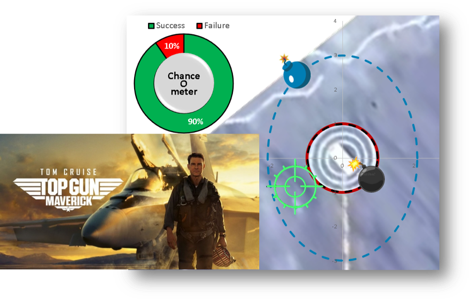
The ChanceOmeter is just a pie chart driven off of two cells on the Calculations page. The green segment is based on a cell created with the Chance of Whatever button in ChanceCalc, and the red segment is simply 1 minus the other cell.

The BayesOmatic is more complicated, especially for people who do not understand Bayesian analysis, which is approximately everybody. It calculates the chance of various outcomes of the mission given specified conditions. For example, we can calculate the chance that the mission would succeed given the malfunction of both targeting lasers. 

How it works

Bayes Theorem states that

Probability of event A given event B = Probability of events A and B ÷ Probability of event B

This can be viewed geometrically as the chance that a dart is in region A given that you know it has already hit B as shown.  This is elementary to do in a SIPmath model by creating Boolean (0/1) variables that signify that A has occurred, B has occurred, and that A and B have both occurred. This creates three ranges on the PMTable sheet, let’s call them A, B, and A_and_B. Because the results of the 10,000 trials are always live in the Data Table, it is easy to perform Bayesian analysis on the fly and the formula above is simply:

Probability of event A given event B = SUM(A_and_B)/SUM(B)

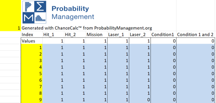
The actual Top Gun Data Table is shown above. Note that targeting laser 2 failed on trial 9.

The User Form

This model sets up the Boolean variables using user forms on the Top Gun sheet to drive formulas on the Calculations sheet. Even I don’t remember how I did this, but I remember where I did this, which should be enough for you to figure it out on your own.

The user controls were created with the Combo Box Form Control available on the Developer Ribbon (which must be made visible under File, Options, Customize Ribbon.) They interact with cells AF47 to AI52 on the Top Gun Sheet.

The cells above are interpreted by a bunch of formulas I hope you can figure out on the Calculations sheet located as shown below.

Note that there is a second copy of our new trial control on this sheet so you can select individual trials as you figure out the formulas above.

Bayesian Inversion

It is also easy to do what is known as Bayesian inversion. Suppose you’re back on the deck of the carrier after a successful mission, and the Maintenance Chief says: “Did you realize that both lasers malfunctioned?” “Impossible,” you say. Well, not exactly. There is a 2 tenths% chance as shown below. To understand the difference, return to the dart. It should be clear from the figure that the chance of hitting in blue given that you hit in yellow is greater than the chance of hitting in yellow given that you hit in blue.

Copyright © 2023 Sam L. Savage

TOP GUN: MAVERICK A WALK IN THE PARK OR MISSION IMPOSSIBLE?

TOP GUN: MAVERICK

A WALK IN THE PARK OR MISSION IMPOSSIBLE?

By John Button, Connor McLemore, and Sam Savage

Presuming the producers maintain this pace, we can barely wait for the 2058 release, when a 96-year-old Tom Cruise at the controls of the only remaining aircraft on Earth, his own WWII P51 Mustang (which appeared in Maverick) flies through a hail of anti-matter death particles to save the planet from the descendants of Chat GPT.

Free Excel Simulation and User’s Guide available at

ProbabilityManagement.org and The Military Operations Research Society

Overview

In the 2022 film sequel Top Gun: Maverick, Tom Cruise returns to the screen as Pete “Maverick” Mitchell, one of the Navy’s top aviators, to lead a specialized and seemingly impossible mission.

The screenwriters must have bent over backwards to come up with a mission that required actual humans to fly less-than-state-of-the-art aircraft at the edges of their aerobatic envelopes for a sustained period. But hey, that’s Hollywood, and we loved it as much as the original 1986 version. Presuming the producers maintain this pace, we can barely wait for the 2058 release, when a 96-year-old Tom Cruise at the controls of the only remaining aircraft on Earth, his own WWII P51 Mustang (which appeared in Maverick) flies through a hail of anti-matter death particles to save the planet from the descendants of Chat GPT.

But at ProbabilityManagement.org, we have our own seemingly impossible mission: to foster chance-informed thinking. So, in spite of being big fans of the movie, we had to ask the logical question, “How would you calculate the chances of Maverick actually pulling this off?”

Armed only with ChanceCalc, we were concerned that we could either build a trivial model that taught little, once we grabbed your attention with Tom Cruise, or a complex model that would make your eyes cross. However, after consultation with Connor McLemore, our chair of National Security Applications, and a graduate of the Navy’s actual Top Gun program, we believe we have developed a stealth model that delivers a payload of insight.

And what a great way to kick off the new Community of Practice (CoP) of Probability Management at the Military Operations Research Society as discussed in my recent blog. You can find the Top Gun ChanceOmeter and other examples on the Models tab of the MORS CoP page as well as on our own Military Readiness page.

Mission Description

“Maverick” has been authorized by the President, and tasked by the Pentagon, to lead a specialized strike team to take out the enemy’s illegal uranium plant before it is fully operational and make it back safely to tell the story. Just a walk in the park, right? Well, not quite.

The plant sits in an underground bunker, surrounded by two mountains. The strike mission in the movie is based on four complicating factors:

• Hitting a very small target (three meters wide,) two consecutive times

• at a very precise angle,

• in a very steep valley,

• in a GPS-jammed environment.

The attack strategy calls for two sections (a.k.a, ‘2-ships’), with F/A-18E flight leads (Maverick and Rooster) and F/A-18F wingmen (Phoenix w/ Bob and Payback w/ Fanboy). Each aircraft pair will fly in a welded wing formation with one plane aiming the targeting laser and the other plane delivering the weapon. Each pair must accomplish one of two dependent actions:

• F-18 Pair 1: The first pair will breach the reactor by dropping a laser-guided bomb on an exposed ventilation hatch. (This will create an opening for the second pair.)

• F-18 Pair 2: The second team will deliver the kill shot.

Model Overview

We suggest that you download the free Excel model and user’s guide for more detail. [1] Here we will summarize the model and its development. It was created with ChanceCalc, from ProbabilityManagement.org, and runs 10,000 trials per keystroke in native Excel. Simply set the parameters involving pilot proficiency and targeting laser dependability on the left side of the screen and read the chance of success off the ChanceOmeter. You may also cycle through each of the 10,000 trials. This model makes use of the powerful Data Table in Excel, which has the potential to bring interactive simulation to tens of millions of users.

Model Development

As mentioned above, two weapons are required: one to destroy the protective ventilation hatch, and the other to destroy the target. Of course, the aim of the weapons is not 100% accurate, and the bombs will land in ellipses that reflect the proficiency of the pilot. So, we started with this aspect, which we thought would be easy to model. It wasn’t, and the next thing we knew we were wading through mathematical formulas on the Internet that would make your head spin (see the user’s guide for references if you are into statistics). But after that was mastered, Connor pointed out that the dispersion error is virtually nil with laser targeted weapons. However, we were saved again by the script writers’ back bends. One of the targeting lasers actually malfunctioned in the movie so we could simulate malfunctions in our model and use the wider dispersion in that case. This led eventually to the BayesOmatic, which was far more consequential than being able to model dispersion ellipses.

The BayesOmatic

This feature is an automated way to perform a powerful technique known as Bayesian Analysis. A future blog will be devoted to this concept, and you can also read more in the User’s Guide. Here we will simply describe how to use this feature to calculate the conditional chances of various events.

For example, with the original model settings, the chance of mission success was about 89%. We can use the BayesOmatic to estimate the chance of success given that both targeting lasers malfunctioned. We see that it is reduced to only 22.8%.

Or how about if you make it back to the deck of the carrier after a successful mission, and the Maintenance Chief says: “Did you realize that both targeting lasers malfunctioned?” “Impossible,” you say. Well not exactly. There is a 2 tenths% chance as shown below.

How can these be so different? Depending on the dispersion ellipses given targeting laser malfunction it is not surprising that the chance of success would be reduced to about 23%. But how about the 0.2%? Well the chance that both lasers malfunction is 10% x 10% = 1%. And we are asking what the chance is that happened, and we also had a successful mission. The bottom line is that Bayesian Analysis is powerful and underutilized, and we that this inspires some of you to learn more about it.

Remember that the Top Gun ChanceOmeter runs in native Excel and requires no macros or add-ins. So, feel free to send it to everyone you know. Or, better yet, send it to everyone you don’t know!

References:

[1] We suggest downloading the model and documentation at either the MORS CoP page or our Military Readiness page.

Copyright © 2023 John Button, Connor McLemore, and Sam Savage

Silicon Valley Bank - The Sound of Two Hands Clapping Incoherently?

Matthew Raphaelson, our Chair of Financial Applications, was my student at Stanford in 1991. He went on to become CFO of a multi-billion-dollar organization at which he pioneered probabilistic thinking. He points out that SVB no doubt had stochastic models of both their investments and depositors. Individually each of these models might have indicated smooth sailing. When the right hand doesn’t know what the left hand is doing, but they both happen to be clapping, there is no sound. Had both models been driven by same stochastic library of interest rates, perhaps management might have noticed that the same event that would trigger large losses in their investments would trigger large withdrawals by their depositors, which is what put them under.

by Sam L. Savage

Banking, Liquidity, and the Likelihood of Simultaneous Failures

by Matthew Raphaelson - Download Bank Risk Model

Banks – like people – can survive all sorts of health issues for months, even years.  A liquidity crisis, however, can be fatal to banks – and people – within days.  For banks, liquidity means access to money, and they take great measures to have ready pools of funds to cover any emergency.  So how did Silicon Valley Bank (SVB) in effect die of thirst?

Banks collect deposits from individuals and businesses and lend those deposits to other individuals and businesses to make money on the interest. Money lent out is not available to depositors; it cannot be withdrawn at the ATM or used to pay bills.  So, banks reserve a portion of deposits not lent – this is known as liquidity.

Banks understand liquidity well, based on years of experience with patterns of customer behavior.  They know paydays, when social security checks arrive, when rents are due.  Since they do not earn much interest on liquidity, banks have a profit motive to maintain no more liquidity than is required by regulation.

Figure 1.  Hypothetical bank liquidity model: “magical thinking” results in a modest liquidity cushion (difference between red line and blue line)

This model of bank liquidity works so long as customers continue to behave predictably, that nothing causes too many of them to withdraw all their money all at once.

The underlying assumption is that bank customers are a varied lot, and respond differently to whatever is going on in the economy.  What if this assumption does not hold, if the entire customer base is sensitive to a single economic indicator, such as interest rates?  Such was the case with SVB and its tightly-knit VC and tech customer base.

During a decade of what Harvard professor Mihir Desai calls “magical thinking”:

…the assumption that favored conditions will continue forever without regard for history. It is the minimizing of constraints and tradeoffs in favor of techno-utopianism and the exclusive emphasis on positive outcomes and novelty. [1]

Venture capital (VC) and tech funding increased by a factor of 10. At the same time, and for the same reasons, SVB deposits also increased by a factor of 10. When the Fed increased interest rates in 2022 and shattered the illusion of magical thinking, the cycle reversed – by Q4 2021 VC funding had fallen 66% from a year earlier. [2] SVB deposits fell $25 billion, or between 10-15%.

Figure 2.  Once the interrelationship between interest rates, customer liquidity and bank liquidity is captured, it is clear the “magical thinking” liquidity model vastly under-estimates the true liquidity requirement (difference between red line and black line)

By itself, an interest rate-driven reduction in liquidity of less than 15% should not be fatal for SVB. Unless there was another interest rate-driven problem somewhere else in the bank. Unfortunately…there was.

Like many banks, SVP used deposits to invest in long-term bonds. These bonds pay higher interest, so the banks make more money.

When interest rates rise, these bonds lose value. This has been widely and correctly reported in the media, and the “unrealized losses” [3] look frighteningly large…in SVB’s case, large enough to wipe out all its capital.

Less well reported is what happens when the losses remain unrealized, meaning the bank is not forced to sell the bonds before they mature. Suppose the rest of the bank’s balance sheet is more valuable as interest rates rise. This occurs when most loans are variable rate and most deposits are fixed rate – in which case the bank can increase profits, despite the bond portfolio. This was exactly how SVB constructed its balance sheet.

SVB management may have believed that the bank was more profitable as interest rates rose…as long as there wasn’t some liquidity problem that forced the bank to sell bonds.

Figure 3a.  Hypothetical bank with high unrealized losses but no additional liquidity risk.  The bank has enough capital to absorb actual losses.

But there was a liquidity problem…a big one. The same factor – rising interest rates – which caused an unrealized losses in the bond portfolio simultaneously triggered the very liquidity problem that crystalized unrealized losses into actual losses.

Figure 3b.  With interrelationships between interest rates, customer liquidity, bank liquidity, and bond values captured, insolvency is imminent.

If this weren’t bad enough, a few influential tweeters raised the alarm about SVB and may have unleashed a herd instinct among the close-knit customer base. The initial $25 billion of liquidity drain was followed by a $40 billion bloodletting in a period of a couple of days, which was not survivable.

Based on our experience, it would not be surprising if SVB had sophisticated interest rate risk models and liquidity coverage models that were nonetheless incoherent. Such models typically envision what would happen in hundreds or thousands of future parallel universes. Incoherence would occur if both models failed to capture the impact of rising interest rates in a consistent and coordinated way – one model can’t be in a universe of rising rates while the other is in a universe of stable or falling rates.

Summary: The Plight of Silicon Valley Bank

1. SVB’s bond portfolio was exposed to losses from rising interest rates, and the bank’s view on liquidity may have been influenced by magical thinking. Neither issue is unique to SVB.

2. SVB catered to an undiversified customer base whose own liquidity was weakened by rising rates. This does appear to be unique to SVB.

3. SVB apparently did not understand the extent to which rising interest rates would simultaneously result in unrealized losses and a liquidity crunch which would cause those losses to materialize.

This is illustrated in figure 3b – the distribution of customer withdrawals has “herded” to the right, triggering asset sales and high losses, and likely insolvency.

4. As financial markets recognized SVB’s dilemma, SVB’s close-knit customer base whipped into a panic via social media, accelerating the bank’s demise.

References:

[1] Mihir Desai, “The Crypto Collapse and the End of the Magical Thinking That Infected Capitalism,” The New York Times, 16 January 16, 2023

[2] EY.com, “Q4 2022 Venture Capital Investment Trends

[3] Unrealized losses are the losses that would occur if the assets are sold.  If the assets are not sold, there are no losses.  For example, suppose you bought a house for $250,000 and in today’s market the value was only $200,000.  If you sold the house today, you would lose $50,000.  But if you don’t sell, you don’t lose.

Copyright © 2023 Sam L. Savage

MORS Announces a Community of Practice in Probability Management

by Sam L. Savage

I am thrilled to announce that the Military Operations Research Society, MORS, has established a Community of Practice (CoP) in the discipline of Probability Management to be headed up by long-time supporters, Phil Fahringer of Lockheed Martin and Max Disla of the Defense Contract Management Agency (DCMA). I also wish to thank MORS members, Connor McLemore and Shaun Doheney whose efforts contributed to establishing the CoP. Learn more about the MORS Probability Management Community of Practice.

The CoP webpage has a Models tab with military operations research examples including the Top Gun ChanceOmeter which I will describe in a future blog.

For now I want to say a few words about the field of Operations Research, and my affinity for it. Operations Research, OR as it is called for short, grew out of the mathematics applied to the unprecendented logistical problems imposed by WWII. I was exposed to the field prenatally in 1944 when my dad was working at the Statistical Research Group run out of Columbia University. This group worked on such problems as whether a fighter should be armed with six 50 calibre guns or eight 30 calibre guns. One of the most famous ideas, today called survivorship bias, came from statistician Abraham Wald. He noted that when assesing battle damage on returning bombers you should not reinforce the places with lots of bullet holes because these were the planes that came back. Instead you should reinforce the places where you never saw a bullet hole!

Operations Research spawned many powerful analytical techniques in use today. The non-military version became known as Management Science, and today both of these have been subsumed under Analytics. There are academic departments of Operations Research at Berkeley, Columbia, Cornell, and Princeton, among others, and the one with which I am most familiar, at the Naval Postgraduate School (NPS) in Monterey, CA.

ProbabilityManagement.org has greatly benefitted through its contacts with NPS and a number of our volunteers have OR degrees from NPS. To learn more visit our Military Readiness page.

Copyright © 2023 Sam L. Savage